Section 3.6 Modeling Working Group
| Science Team Projects with Modeling Components | |
| Goetz-03 | Rogers-01 |
| Fisher-01 | Schaefer-04 |
| Kimball-04 | Schaefer-05 |
| Miller-C-03 | Wullschleger-01 |
|
| |
| Data & Knowledge Gaps |
| Overarching Objectives |
| Approach / Protocol |
| Variables of Interest |
| Remote Sensing Integration |
| Domain |
| Links to Other Working Groups |
| References |
Data & Knowledge Gaps
The Arctic-Boreal Region (ABR) is the source of among the largest uncertainties to global climate projections [Koven et al., 2011;IPCC, 2014; Schaefer et al., 2014; Snyder and Liess, 2014]. Model estimates from both coupled and offline terrestrial biosphere models (TBMs) are orders of magnitude different from one another for ABR soil carbon, exhibit nearly every possible spatial configuration of net carbon sinks and sources across models, and, in general, are poorly parameterized with respect to cold/frozen environment sensitivities [McGuire et al., 2001;McGuire et al., 2012;Fisher et al., 2014] (Figure 1).
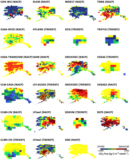
There is a critical need to simultaneously improve ABR model representation and eliminate poor model output to achieve reductions in climate uncertainty. This large spread among models defines the IPCC-type uncertainty for the region, but there are few data with which to benchmark models to guide improvements. This presents a formidable challenge towards addressing the ABoVE Overarching Science Question: how vulnerable or resilient are ecosystems and society to environmental change in the ABR of western North America?
Addressing the Ecosystem Dynamics Objectives focus of ABoVE Phase I research requires an interdisciplinary suite of modeling and scaling capabilities (Figure 2) for studying the key ecosystem indicators: 1) disturbance, 2) flora/fauna and related ecosystem structure and function, 3) carbon pools and biogeochemistry, 4) permafrost properties, and 5) hydrology. We must coordinate data collection activities in Phase I to evaluate and improve model performance in representing, simulating, and scaling the key indicators of these ecosystem dynamics. Moreover, to directly address the definition of multi-model spread uncertainty, it is crucial that multiple TBMs both inform data collection and are improved from the data collected.
Overarching Objectives
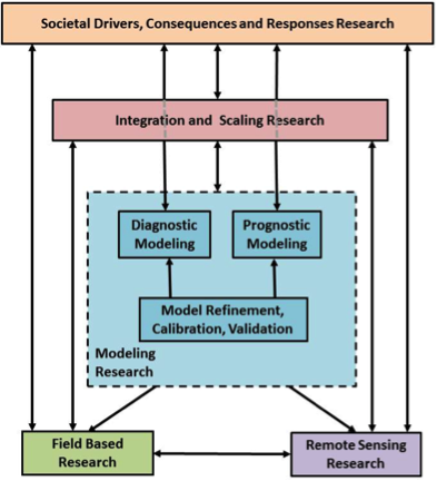 Figure 2. From the ABoVE Concise Experiment Plan (ACEP): modeling research is positioned at the interconnecting center of all ABoVE activities.
Here, our Working Group coalesces a suite of modeling teams and model elements within field- and/or remote sensing-based teams within the ABoVE Science Team to provide a meta-synthesis of TBM requirements for the ABoVE campaign data collection. This includes parameter and structural uncertainties to guide data types, environmental ranges of measurement, and co-measured variables necessary to improve ABR simulations addressing the Tier 2 science questions. The goals of this team-of-teams will be to: 1) use an inter-comparison of a suite of TBMs to identify critical data gaps for informing and prioritizing ABoVE remote sensing and field data collection; 2) develop and employ a flexible and consistent data integration, simulation, and evaluation framework for ABoVE modeling research; and, 3) build the foundational capacity of investigators, datasets, modeling tools, and benchmarking targets for addressing the ABoVE Ecosystem Services Objectives and other scaling research needed for the subsequent Phase II research activities.
The overarching objective is to evaluate and improve model performance of ABR ecosystem dynamics focusing on critical data gaps in initializing, driving, and validating process-based simulations for the ABoVE domain.
Approach/Protocol
The Modeling activities included in ABoVE Phase I research span a large domain of complexity and approach: I) global TBMs that attempt to encompass a large suite of interconnecting processes; II) local scale ecosystem models focused on particular components of the terrestrial biosphere (e.g., trees, fire, permafrost); III) statistical upscaling approaches for extrapolating in situ measurements to construct regional datasets; and, IV) remote sensing retrieval algorithms to construct biophysical data products from remote sensing measurements. Here, we focus on the first two types with the key definition for inclusion being the study of ecosystem process; the ultimate goal is to improve multiple TBMs throughout the international community.
Goal 1 (Year 1): foundational
1A. Initial model inter-comparison and evaluation: use existing TBM simulation results to compare and evaluate models against existing field and remote sensing data on each of the 5 ABoVE ecosystem dynamics indicators.
1B. Identify and prioritize data gaps: use the TBM inter-comparison results to analyze sensitivities to driver data, model structures, and uncertainties in simulating ecosystem dynamics indicators; these results will contribute to the ABoVE data collection Implementation Plan to ensure data are collected that are designed to reduce model uncertainties.
Goal 2 (Year 2): structural
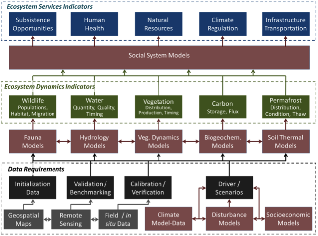 Figure 3. From the ABoVE Concise Experiment Plan (ACEP). This figure diagrams the full modeling plan stated as required by ABoVE. The modeling elements for ABoVE Phase I will fully complete 2 out of the 3 components: the Data Requirements (black) and the Ecosystem Dynamics Indicators (green).
2A. Data assembly and organization: work with the CC&E Office/ABoVE Science Cloud and selected Science Team to assemble and organize initialization, driver, calibration, and evaluation datasets in operable and consistent formats to support modeling research.
2B. Modeldata integration and refinement: modeling teams will begin to prepare their models for ingestion of ABoVE data, especially with respect to remote sensing data.
Goal 3 (Year 3): synthesis
3A. Simulation and benchmarking framework: incorporate relevant newly collected ABoVE datasets into a community-endorsed benchmarking system (e.g., ILaMB; Permafrost Benchmark System) [Randerson et al., 2009]; the benchmarking data and system, which we will optimize for ABoVE research, will be made available to the modeling community to confront their models against ABR-specific variables and use the framework for iterative testing and refinement of key model parameters and structural formulations.
3B. Evaluate model progress: perform an update of the initial model inter-comparison and evaluation using ABoVE models and data; improvements can be assessed in terms of how the data collected, and model refinements made, during ABoVE have contributed to reduced uncertainty and improved simulation of the key ecosystem dynamics indicators.
3C. Prelude to Phase II modeling research: synthesize “lessons learned” from this project to guide preparations for modeling research that addresses the ABoVE Ecosystem Services objectives; this includes new and continued field and remote sensing data collections, model refinements, and opportunities for collaboration across modeling teams as well as integration with social system models and other ABoVE Phase II research activities.
Model outputs will be compared to and evaluated against existing field and remote sensing data among each of the 5 categories of ABoVE ecosystem dynamics indicators (vegetation, carbon, permafrost, water, wildlife/habitat; Figure 3). These include: habitat distribution and connectivity (Wildlife); the full terrestrial water cycle—precipitation/snow, evapotranspiration, soil moisture, groundwater, runoff, storage change (Water); ecosystem/vegetation functional characteristics, pre-cursers to fire, and regrowth (Vegetation); soil carbon stocks and changes, ecosystem carbon fluxes, environmental sensitivities (Carbon); and seasonal freeze/thaw (Permafrost).
Detailed Modeling Activities
While most of the 5 ABoVE ecosystem dynamics categories and variables are encompassed within full TBMs, ABoVE modeling activities also include model analyses and developments focused on targeted variables or ecosystem dynamics.
A suite of models will be used to improve the representation of snowpack evolution (SnowModel) [Prugh], coupled permafrost and hydrology (SUTRA4.0) [Striegl], and other hydrologically-focused landscape-scale interrelationships (PFLOTRAN, ATS, TCF-PWBM, CanFIRE) [Wullschleger; Kimball; Bougeau-Chavez].
Tree-level modeling of forest productivity and demographics, using the forest gap models UVAFME and ED2, will address how mixed species stands are responding to climate and environment specifically trends in boreal tree mortality, as well as potential range expansion across the ABoVE domain, which is an important component of the ABR [Shuman; Rogers; Goetz; Eitel; Vierling; Moghaddam]. Shifts in productivity, diurnal cycle patterns, or species dominance are a result of the interaction of temperature, soil characteristics, land surface hydrology, and species tolerances, but species-level responses vary spatially and temporally. These impact habitat use and harvest models for animals such as Dall sheep [Prugh; Boelman].
The rate of which the land surface re-sequesters carbon following fire will be assessed, taking into account species-level succession and a suite of other local/regional drivers. Fire processes capturing fuel loading, burn severity, and land cover influence will be modeled and improved through focused research activities [Bourgeau-Chavez; Rogers].
We will use satellite and airborne observations to evaluate modeled CO2 and CH4 fluxes over the ABoVE domain [Kimball; Miller; Moghaddam]. An in depth evaluation of process level representation of land-atmosphere carbon exchange will be conducted for a suite of TBMs, including CASA, TDF, CLM, PVPRM, CARDOMAM, and ED2. The goals of these modeling activity are: I) to link changing surface conditions, freeze-thaw regimes, soil moisture, and open water inundation with variable controls on the net ecosystem carbon budget; II) to test the hypothesis that relatively warm and wet years result in the highest positive NEP flux totals; and, III) investigate the impact of permafrost soil dynamics and surface soil moisture information on regional carbon flux simulations. We will focus on sub-grid scale processes affecting carbon flux estimates, while incorporating regional model enhancements representing wildfire disturbance recovery and wetland CH4 emissions. Light-use efficiency (LUE) modeling will be evaluated in depth using satellite indices [Gamon].
Table 1. Benchmarking data to be used in our MoDIF project spans the full range of Indicators for ABoVE ecosystem dynamics.
| Variable | Dataset | Coverage |
| Carbon Dynamics | ||
| NDVI, EVI, LAI, fAPAR, NPP | MODIS | Global; weekly; 2002-2013 |
| Soil Carbon Stocks / Depth | Pedons | Regional; static; 100 km |
| Soil Carbon Residence Time | Incubations | Local; static; 1 m |
| CO2 fluxes | AmeriFlux, MPI-BGC | Local/global; hourly; 1 km |
| CO2, CH4 concentration | CARVE, GOSAT, OCO-2/3, SCIAMACHY | Regional/global; weekly; 1-3 km |
| Biomass | ICESat/GLAS, G-LiHT, GEDI, CFS | Regional/global; static; 0.25-1 km |
| Canopy height | ICESat/GLAS, G-LiHT, GEDI | Regional/global; static; 1 km |
| Water Dynamics | ||
| Soil moisture | SMAP, SMOS, ISMN | Local/regional/global; <weekly; 3-9 km |
| Evapotranspiration | MODIS, ECOSTRESS | Regional/global; <weekly; 0.05-1 km |
| Total Water Column | GRACE | Global; monthly; >100 km |
| Snow characteristics | NASCN, NOAA Snow Cover, MODIS | Regional/local; weekly-annually; 1 km |
| Energy Dynamics | ||
| Soil, surface temperature | GTN-P, BOREAS, MODIS | Local/regional/global; weekly-static; 1 km |
| Freeze/thaw | SMAP | Regional/global; <weekly; 3 km |
| Active layer depth | InSAR, CALM/GTN-P | Regional; static; 1 m |
| Albedo | MODIS, VIIRS | Global; weekly; 1 km |
| Fire counts, burnt area | MODIS | Global; weekly; 1 km |
| Net radiation | MODIS | Global; weekly; 1 km |
Remote Sensing Integration
Model outputs will coincide with remote sensing data and products for: phenology (MODIS NDVI, EVI, fAPAR) [Huete et al., 2002; Myneni et al., 2002], GPP and NPP (MODIS) [Zhao et al., 2005; Beer et al., 2010], fire (MODIS) [Giglio et al., 2003], albedo (MODIS) [Jin et al., 2003], biomass (ICESat/GLAS) [Yu et al., 2011], canopy height (ICESat/GLAS) [Simard et al., 2011], evapotranspiration (MODIS) [Fisher et al., 2008; Mu et al., 2011], soil moisture (SMOS) [Kerr et al., 2001], total water storage and derived groundwater (GRACE) [Rodell and Famiglietti, 2002], and land surface temperature (MODIS) [Wan, 2008] (Table 1). Additional remote sensing products developed by the ABoVE Science Team during Phase I may be used as well; consideration of relevance and quality will be given as they are developed.
- Modeling activities encompass the entire ABoVE Domain (Figure 4).
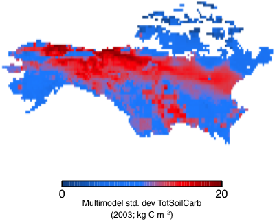 Figure 4. The ABoVE Domain, as represented by model uncertainty in soil carbon stocks.
Links to Wildlife and Ecosystem Services
- How is fauna responding to changes in biotic and abiotic conditions, and what are the impacts on ecosystem structure and function?
- TBMs do not typically explicitly represent faunal characteristics; however, habitat distribution and connectivity are represented in TBMs, and the models will be evaluated for these characteristics.
- How are environmental changes affecting critical ecosystem services – natural and cultural resources, human health, infrastructure, and climate regulation – and how are human societies responding?
- This question will not be directly addressed in the scope of this Working Group. In the final year, we will provide direction on how to address this goal from a modeling perspective in ABoVE Phase II (Figure 5).
Links to Vegetation Properties, Processes & Dynamics
- How is flora responding to changes in biotic and abiotic conditions, and what are the impacts on ecosystem structure and function?
- TBMs are mature in representing floral changes to environmental conditions through structure and function, yet uncertainties remain large in the ABR. Models will be evaluated against remotely sensed structural observations (e.g., ICESat; GEDI will be linked at a later stage) [see, for example, our TBM ecosystem structural benchmarking work in Kelley et al., 2012] and functional observations (e.g., MODIS; OCO-2/3 will be linked at a later stage) [e.g., Parazoo et al., 2014]. A critical evaluation will assess decadal greening/browning and biome expansion/contraction (e.g., AVHRR).
- Individual-scale tree models target this question directly, and lessons learned can be aggregated and incorporated into PFT-based TBMs.
Links to Fire Disturbance
- What processes are contributing to changes in disturbance regimes and what are the impacts of these changes?
- Fire (and, to a lesser extent, insects and pathogens) is included in many TBMs. While fire sparks are difficult to model in an exact sense (they are typically represented as probabilistic in prognostic models), the pre-cursers to fire and extent (fuel load, quality, distribution, moisture) and regrowth dynamics should be captured in models. TBMs will be evaluated in their representation of fire pre-cursers prior to remotely sensed fire observations and regrowth dynamics relative to vegetation remote sensing observations. Moreover, models will be evaluated for burned area/frequency over decadal temporal integration periods. Finally, burn severity, as linked to the pre-cursers, will be evaluated as a high quality burn severity dataset will be produced in ABoVE.
- While spatial data on wildfire occurrence, extent, and severity are readily available across Alaska and Canada, information on other important disturbances such as insects, pathogens, rapid thaw events (thermokarst) and land use change are not. As modeling representatives, we will engage with the ABoVE Science Team early in the campaign planning process to solicit existing and new data and research activities related to the more comprehensive suite of disturbance types from investigators working across the various Research Areas of the Domain.
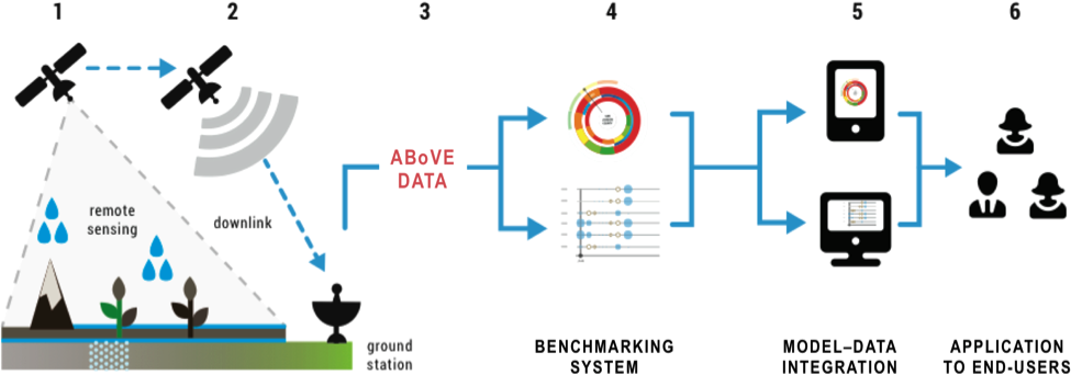 Figure 5. Overview flow diagram of the modeling activities. ABoVE field and remote sensing data are collected (1), processed (2), delivered to the ABoVE Science Cloud (3), integrated into a benchmarking system (4), interfaced with multiple models for model improvements (5), and linked as Ecosystem Services (Phase II) to end-users (6).
Links to Carbon & Biogeochemistry Dynamics
- How are the magnitudes, fates, and land-atmosphere exchanges of carbon pools responding to environmental change, and what are the biogeochemical mechanisms driving these changes?
- From a climate change standpoint, this question is arguably the most important component that TBMs should represent well. But, as demonstrated in McGuire et al. [2012] and Fisher et al. [2014], TBMs suffer in representing soil carbon pools well. We will evaluate with critical priority TBM ability to capture soil carbon stocks and changes, and environmental sensitivities leading to changes.
Links to Hydrology & Permafrost
- What processes are controlling changes in the distribution and properties of permafrost and what are the impacts of these changes?
- Modeled soil thermal and hydraulic properties will be evaluated against the NASA MEaSUREs 25 km historical freeze/thaw product [Kim and Lee, 2012]. Some of the uncertainty with respect to modeled permafrost is outside the control of model parameterization, instead lying in the uncertainty inherent in the forcing data (e.g., temperature, radiation). Nonetheless, models will be evaluated in their qualitative ability to represent seasonal dynamics of freeze/thaw.
- What are the causes and consequences of changes in the hydrologic system, specifically the amount, temporal distribution, and discharge of surface and subsurface water>
- TBMs have fully coupled hydrological cycles, and can thus be evaluated directly against remotely sensed hydrological observations. SMOS can be used for near-historical soil moisture; SMAP will be used for higher accuracy and resolution. GRACE will be used to evaluate the anomaly in total water column represented in TBMs. MODIS, and later ECOSTRESS, will be used to evaluate the evapotranspiration from TBMs.
References
Beer, C., M. Reichstein, E. Tomelleri, P. Ciais, M. Jung, N. Carvalhais, C. Rödenbeck, M. A. Arain, D. Baldocchi, G. B. Bonan, A. Bondeau, A. Cescatti, G. Lasslop, A. Lindroth, M. Lomas, S. Luyssaert, H. Margolis, K. W. Oleson, O. Roupsard, E. Veendendaal, N. Viovy, C. Williams, F. I. Woodward, and D. Papale (2010), Terrestrial gross carbon dioxide uptake: Global distribution and covariation with climate, Science, 329, 834-838.
Fisher, J. B., K. Tu, and D. D. Baldocchi (2008), Global estimates of the land-atmosphere water flux based on monthly AVHRR and ISLSCP-II data, validated at 16 FLUXNET sites, Remote Sensing of Environment, 112(3), 901-919.
Fisher, J. B., M. Sikka, W. C. Oechel, D. N. Huntzinger, J. R. Melton, C. D. Koven, A. Ahlström, M. A. Arain, I. Baker, J. M. Chen, P. Ciais, C. Davidson, M. Dietze, B. El-Masri, D. Hayes, C. Huntingford, A. K. Jain, P. E. Levy, M. R. Lomas, B. Poulter, D. Price, A. K. Sahoo, K. Schaefer, H. Tian, E. Tomelleri, H. Verbeeck, N. Viovy, R. Wania, N. Zeng, and C. E. Miller (2014), Carbon cycle uncertainty in the Alaskan Arctic, Biogeosciences, 11(15), 4271-4288.
Giglio, L., J. Descloitres, C. O. Justice, and Y. J. Kaufman (2003), An enhanced contextual fire detection algorithm for MODIS, Remote Sensing of Environment, 87(2-3), 273-282.
Huete, A., K. Didan, T. Miura, E. P. Rodriguez, X. Gao, and L. G. Ferreira (2002), Overview of the radiometric and biophysical performance of the MODIS vegetation indices, Remote Sensing of Environment, 83(1-2), 195-213.
IPCC (2014), Climate Change 2014: Impacts, Adaptation, and Vulnerability. Part A: Global and Sectoral Aspects. Contribution of Working Group II to the Fifth Assessment Report of the Intergovernmental Panel on Climate Change, 1132 pp., Cambridge University Press, Cambridge, United Kingdom and New York, NY, USA.
Jin, Y., C. B. Schaaf, C. E. Woodcock, F. Gao, X. Li, A. H. Strahler, W. Lucht, and S. Liang (2003), Consistency of MODIS surface bidirectional reflectance distribution function and albedo retrievals: 2. Validation, Journal of Geophysical Research: Atmospheres, 108(D5), 4159.
Kelley, D. I., I. Colin Prentice, S. P. Harrison, H. Wang, M. Simard, J. B. Fisher, and K. O. Willis (2012), A comprehensive benchmarking system for evaluating global vegetation models, Biogeosciences Discuss., 9(11), 15723-15785.
Kerr, Y. H., P. Waldteufel, J. P. Wigneron, J. Martinuzzi, J. Font, and M. Berger (2001), Soil moisture retrieval from space: the Soil Moisture and Ocean Salinity (SMOS) mission, Geoscience and Remote Sensing, IEEE Transactions on, 39(8), 1729-1735.
Kim, S.-G., and S.-J. Lee (2012), Tomographic analysis of porosity variation in gas diffusion layer under freeze-thaw cycles, International Journal of Hydrogen Energy, 37(1), 566-574.
Koven, C. D., B. Ringeval, P. Friedlingstein, P. Ciais, P. Cadule, D. Khvorostyanov, G. Krinner, and C. Tarnocai (2011), Permafrost carbon-climate feedbacks accelerate global warming, Proceedings of the National Academy of Sciences, 108(36), 14769-14774.
McGuire, A., S. Sitch, J. Clein, R. Dargaville, G. Esser, J. Foley, M. Heimann, F. Joos, J. Kaplan, and D. Kicklighter (2001), Carbon balance of the terrestrial biosphere in the twentieth century: Analyses of CO2, climate and land use effects with four process-based ecosystem models, Global Biogeochemical Cycles, 15(1), 183-206.
McGuire, A. D., T. R. Christensen, D. Hayes, A. Heroult, E. Euskirchen, J. S. Kimball, C. Koven, P. Lafleur, P. A. Miller, W. Oechel, P. Peylin, and M. Williams (2012), An assessment of the carbon balance of arctic tundra: comparisons among observations, process models, and atmospheric inversions, Biogeosciences, 9, 3185-3204.
Mu, Q., M. Zhao, and S. W. Running (2011), Improvements to a MODIS global terrestrial evapotranspiration algorithm, Remote Sensing of Environment, 111, 519-536.
Myneni, R. B., S. Hoffman, Y. Knyazikhin, J. L. Privette, J. Glassy, Y. Tian, Y. Wang, X. Song, Y. Zhang, G. R. Smith, A. Lotsch, M. Friedl, J. T. Morisette, P. Votava, R. R. Nemani, and S. W. Running (2002), Global products of vegetation leaf area and fraction absorbed PAR from year one of MODIS data, Remote Sensing of Environment, 83(1-2), 214-231.
Parazoo, N. C., K. Bowman, J. B. Fisher, C. Frankenberg, D. Jones, A. Cescatti, Ó. Pérez-Priego, G. Wohlfahrt, and L. Montagnani (2014), Terrestrial gross primary production inferred from satellite fluorescence and vegetation models, Global change biology, 20(10), 3103-3121.
Randerson, J. T., F. M. Hoffman, P. E. Thornton, N. M. Mahowald, K. Lindsay, Y.-H. Lee, C. D. Nevison, S. C. Doney, G. Bonan, R. Stöckli, C. Covey, S. W. Running, and I. Y. Fung (2009), Systematic assessment of terrestrial biogeochemistry in coupled climate-carbon models, Global Change Biology, 15, 2462-2484.
Rodell, M., and J. S. Famiglietti (2002), The potential for satellite-based monitoring of groundwater storage changes using GRACE: the High Plains aquifer, Central US, Journal of Hydrology, 263(1–4), 245-256.
Schaefer, K., H. Lantuit, V. E. Romanovsky, E. A. Schuur, and R. Witt (2014), The impact of the permafrost carbon feedback on global climate, Environmental Research Letters, 9(8), 085003.
Simard, M., N. Pinto, J. B. Fisher, and A. Baccini (2011), Mapping forest canopy height globally with spaceborne lidar, J. Geophys. Res., 116(G4), G04021.
Snyder, P. K., and S. Liess (2014), The simulated atmospheric response to expansion of the Arctic boreal forest biome, Climate dynamics, 42(1-2), 487-503.
Wan, Z. (2008), New refinements and validation of the MODIS Land-Surface Temperature/Emissivity products, Remote Sensing of Environment, 112(1), 59-74.
Yu, Y., S. S. Saatchi, U. Seibt, and M. A. Lefsky (2011), Mapping global forest carbon stock, in American Geophysical Union, Fall Meeting 2011, edited, San Francisco.
Zhao, M. S., F. A. Heinsch, R. R. Nemani, and S. W. Running (2005), Improvements of the MODIS terrestrial gross and net primary production global data set, Remote Sensing of Environment, 98, 164-176.